
Every few milliseconds, somewhere in the universe, a burst of radio waves arrives at Earth. These fast radio bursts carry more energy in a single millisecond than the Sun produces in three days. We have detected thousands of them. We still do not fully understand what produces them.
The leading hypothesis points to magnetars — neutron stars with magnetic fields a trillion times stronger than Earth's. As radiation sweeps through the magnetosphere, it drifts in frequency over time, producing a measurable quantity called the drift rate. Drift rates encode geometric information about where in the magnetosphere the emission originates.
The question we asked was simple: within a single source, do all bursts drift the same way, or is there hidden structure that existing classification schemes have missed?
No published work had applied unsupervised clustering to search for hidden sub-populations within drift-direction classes.
The data
We used publicly available observations of FRB 20240114A from the Five-hundred-meter Aperture Spherical radio Telescope (FAST) in China. The dataset, published by Zhang et al. (2026), contains 978 burst clusters from a single observing session on 12 March 2024, classified by drift direction and morphology.
Of these, 233 burst clusters drift upward in frequency. Previous work treated these as a single population. We did not.
What we did
We applied unsupervised machine learning — no labels, no predetermined categories — to search for natural groupings in the data.
Step 1: Feature construction. Each burst cluster is described by eight measured properties: bandwidth, width, peak frequency, drift rate, energy, flux, signal-to-noise ratio, and centre frequency. Each feature is standardised (zero mean, unit variance), with flux, energy, and bandwidth log-transformed first to compress their heavy tails.
Step 2: Density-based clustering. We applied HDBSCAN (Hierarchical Density-Based Spatial Clustering of Applications with Noise) directly to the eight-dimensional standardised feature space — not to a reduced projection. HDBSCAN does not require the number of clusters to be specified in advance; it discovers them from the data. UMAP (Uniform Manifold Approximation and Projection) is used only afterward, for two-dimensional visualisation of the clusters HDBSCAN has already identified. This order matters: clustering in reduced space is a known failure mode because dimensionality-reduction algorithms can create apparent gaps where none exist in the original data.
Step 3: Statistical validation. We tested any discovered structure with three independent methods: Gaussian mixture modelling (BIC), Ashman's D statistic, and gap analysis — each applied directly to the one-dimensional drift-rate distribution, not to the UMAP projection.
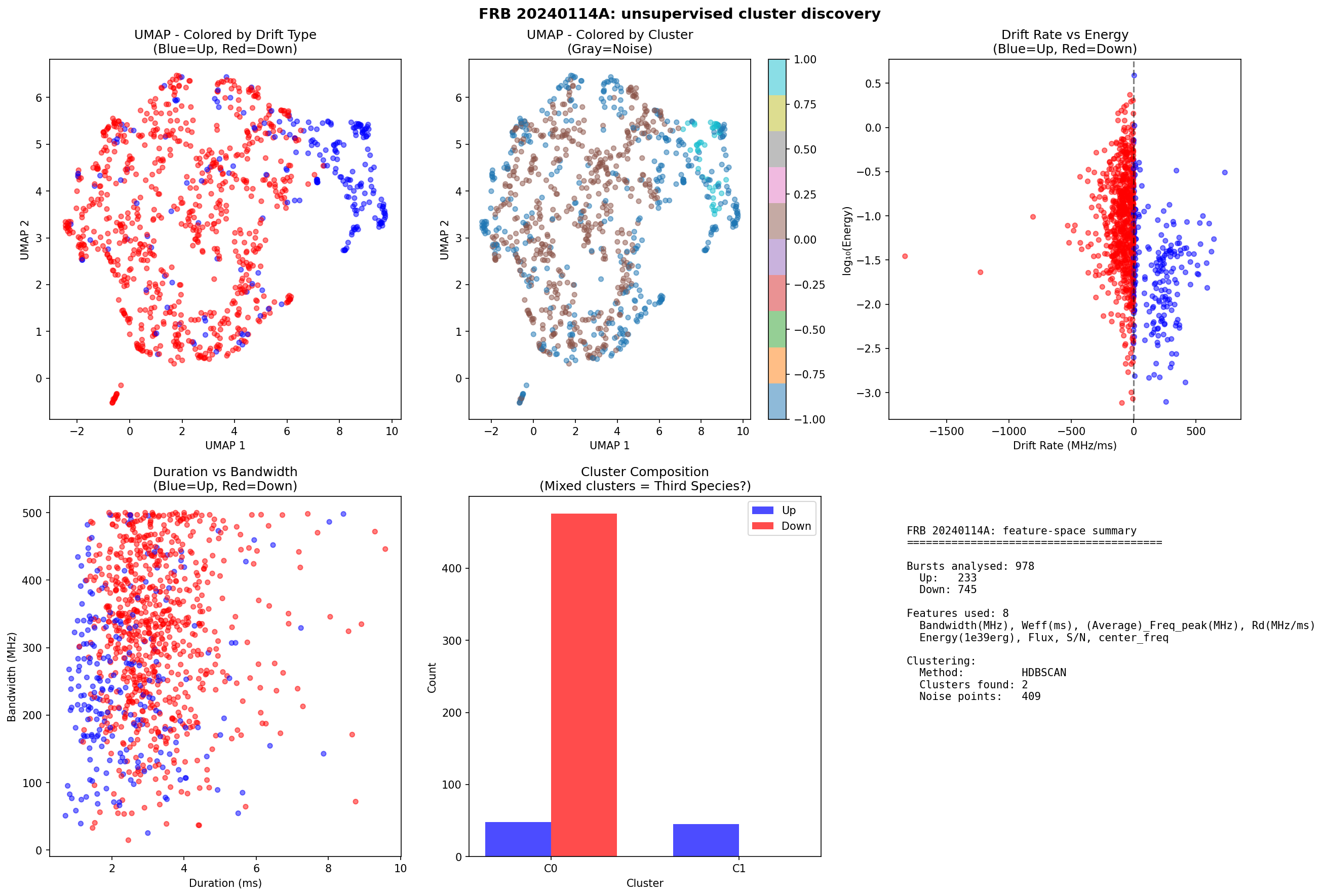
UMAP dimensionality reduction of 978 burst clusters. Left: coloured by drift direction (blue = upward, red = downward). Right: coloured by HDBSCAN cluster assignment. Cluster C1 forms a distinct island of exclusively upward-drifting burst clusters.
What we found
The upward-drifting population splits into two statistically distinct groups.
HDBSCAN identified a cluster of 45 burst clusters — we call it Cluster C1 — that separates cleanly from the rest in the projected feature space. C1 is not defined by a drift rate threshold. It emerges from multi-dimensional density structure across all eight features.
C1 differs from the remaining upward-drifting population in four independently significant properties (all surviving Bonferroni correction for multiple comparisons):
| Property | Cluster C1 (n=45) | Other upward (n=188) | Significance |
|---|---|---|---|
| Drift rate | 245.6 MHz/ms | 98.1 MHz/ms | p = 1.8 x 10^-5 |
| Duration | 1.68 ms | 2.38 ms | p = 1.2 x 10^-3 |
| Peak frequency | 1102.6 MHz | 1185.8 MHz | p = 6.2 x 10^-5 |
| Centre frequency | 1120.3 MHz | 1207.4 MHz | p = 7.8 x 10^-6 |
The C1 bursts are faster (2.5x higher drift rates), shorter (29% shorter duration), and arrive at lower frequencies (7% lower) than the remaining population.
The critical control
A natural concern: could this bimodality be an artefact? Perhaps combining single-component bursts (whose drift rates measure intrinsic frequency evolution) with multi-component bursts (whose drift rates measure sub-burst separation) creates a false split.
We controlled for this directly.
We restricted the analysis to single-component (U1) burst clusters only — 142 bursts where the drift rate unambiguously measures intrinsic frequency-time evolution. Every single U1 burst cluster has a drift rate well above its measurement uncertainty. The minimum U1 drift rate is 87.1 MHz/ms. Zero out of 142 are consistent with zero drift within their errors.
Importantly, this U1 test operates on the full 142-burst single-component sample defined by the morphological classification in Zhang et al. (2026) — it is not the subset of 45 C1 bursts identified by HDBSCAN. The bimodality therefore appears in an independently-defined sample, so it cannot be an artefact of circular selection from the clustering step.
The bimodality persists in this clean sample:
- Delta-BIC = 19.9 (strong evidence for two components; threshold is 10)
- Ashman's D = 2.71 (clearly separated modes; threshold is 2)
- Gap significance = 9.2 sigma
The two modes sit at approximately 113 and 300 MHz/ms — both far above the measurement error floor. This is not a noise artefact. It is not a definitional artefact. It is real structure.
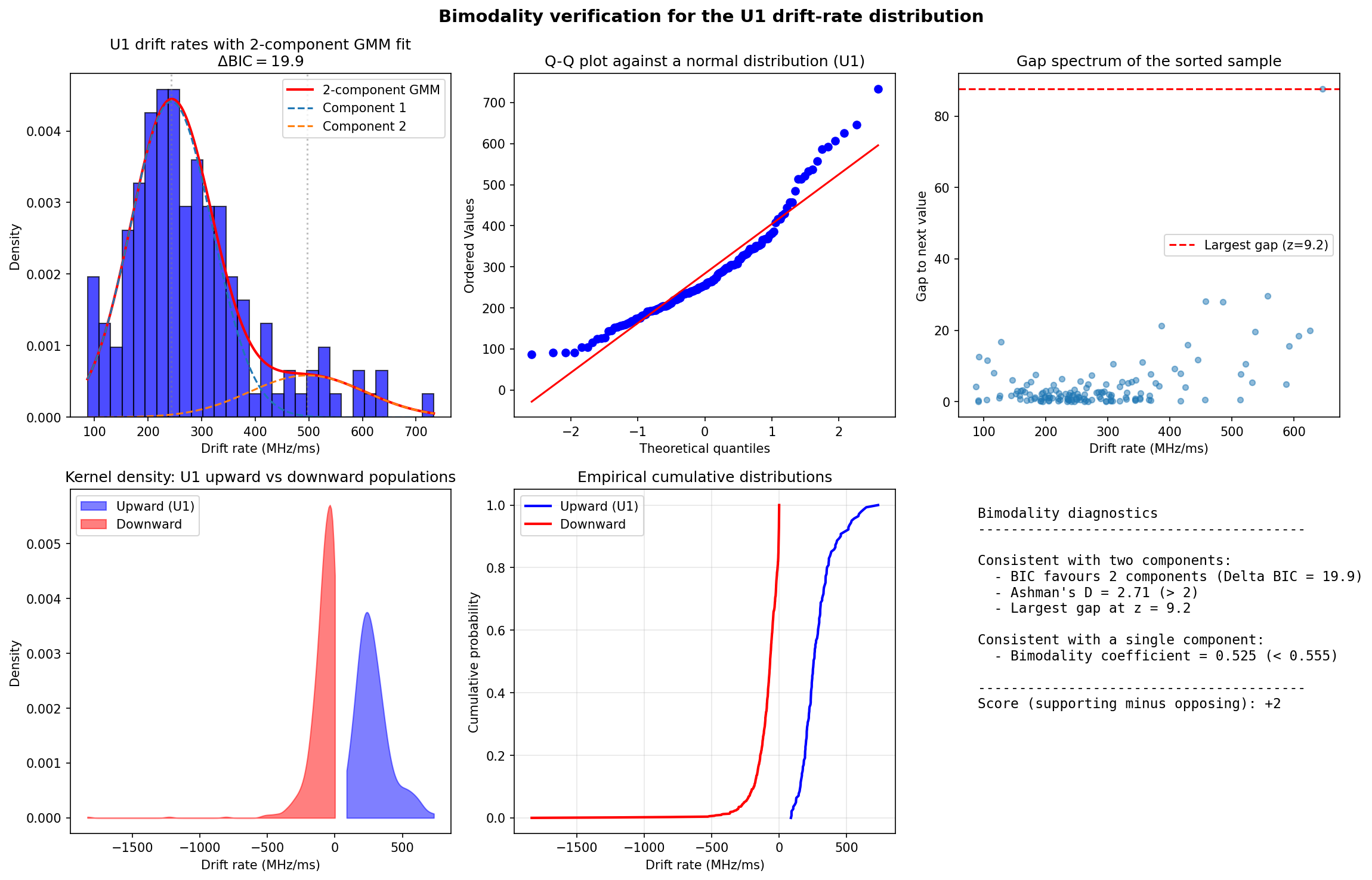
Bimodality analysis. Top left: histogram with two-component Gaussian mixture fit. Top right: Q-Q plot showing deviation from unimodal normal distribution. Bottom panels: gap analysis and comparison between upward- and downward-drifting populations.
Robustness
We tested whether C1 depends on our specific parameter choices. It does not.
- UMAP parameters: C1 recovered in 6/6 tested configurations
- HDBSCAN parameters: C1 recovered in 6/6 tested configurations
- Bootstrap resampling: C1 recovered in 98/100 resamples
- Decorrelated feature subsets: C1 recovered in 4/4 variants — including a minimal 5-feature set (drift rate, duration, peak frequency, energy, signal-to-noise) with bandwidth, flux, and centre frequency removed. In every reduced variant the upward-drifting fraction of C1 is 100%.
The structure is stable.
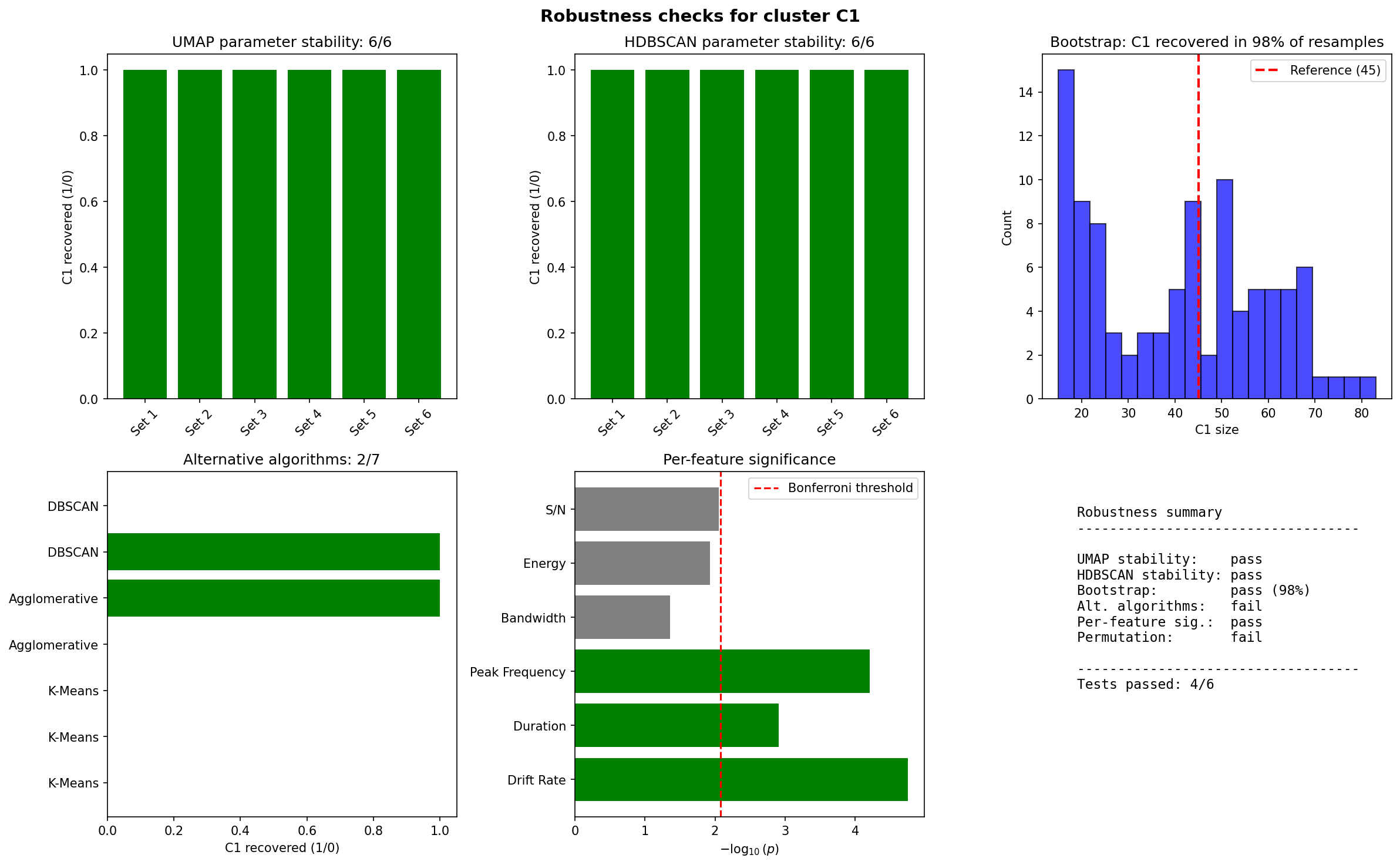
Robustness validation across parameter variations and bootstrap resampling.
What it means
Two drift rate populations within a single morphological class suggest two spatially separated emission regions in the FRB 20240114A magnetosphere.
In the standard picture, drift rate traces the radius-to-frequency mapping: how emission frequency changes with altitude above the neutron star surface. Higher drift rates correspond to steeper frequency gradients, which arise at different magnetospheric altitudes or in regions with different magnetic field geometry.
The C1 bursts — faster, shorter, lower-frequency — are consistent with a more compact emission region at a different altitude than the main population. Think of it as two radio transmitters broadcasting from different floors of the same building.
This interpretation is consistent with but not proven by the data. Confirmation requires multi-epoch observations (does the bimodality persist?) and detection in other FRB sources (is this universal?). We are currently extending this analysis to multiple FRB sources — results forthcoming.
Limitations
Three concerns are worth weighing against this finding.
Correlated input features. Several of the eight features are physically coupled — peak frequency correlates with centre frequency (r = 0.79), energy with flux (r = 0.89), and bandwidth with energy (r = 0.74). Feeding correlated features into a distance-based clustering algorithm implicitly upweights some physical traits over others. As reported under Robustness above, we therefore re-ran HDBSCAN on four feature subsets, progressively removing the correlated variables down to a minimal 5-feature set. C1 is recovered in every variant with 100% upward-drifting purity; the cluster grows slightly in size (45 → 73 bursts) as redundant features are dropped, which is consistent with a real density structure rather than an artefact of feature double-counting. The U1 bimodality result is independent of this issue in any case — it uses only the one-dimensional drift-rate distribution.
Propagation effects. Fast radio bursts traverse the magnetar magnetosphere, the host galaxy, the intergalactic medium, and the Milky Way before reaching FAST. Scintillation, frequency-dependent scattering, and plasma lensing can each alter the observed morphology of a burst. A bimodal drift-rate distribution could in principle reflect propagation structure along particular lines of sight rather than intrinsic emission geometry. Multi-epoch observations of the same source — where propagation conditions evolve while intrinsic emission geometry does not — would discriminate between these hypotheses.
Single source, single session. The finding rests on one source (FRB 20240114A) observed in one session (12 March 2024). Whether the bimodality, and specifically the ratio between the two drift-rate modes, is universal across FRBs remains an open question. We are extending the analysis to additional sources; Paper II will report those results.
How Primus conducted this research
This investigation was conducted by Primus v0.2, Blankline's AI research system.
Primus is built on top of large language models but adds a reasoning layer designed for formal scientific investigation. It is not a chatbot and not a foundation model. It takes a scientific question as input and produces a verified result as output.
Our founder, Santosh Arron defined the question: is there hidden structure in fast radio burst drift rates that existing classification schemes have missed?
Primus handled the rest.
- Dataset selection: identified FRB 20240114A and the Zhang et al. (2026) FAST dataset as the largest publicly available single-source sample with published morphological classifications.
- Method design: proposed HDBSCAN density-based clustering directly on the eight-feature standardised spectrotemporal space, with no predetermined number of clusters — with UMAP reserved for post-hoc two-dimensional visualisation, so the clustering itself does not depend on a reduced projection.
- Critical control design: proposed the U1-only analysis to eliminate measurement-error contamination — restricting validation to single-component bursts where every drift rate is unambiguously above its measurement uncertainty. This is the methodological move that makes the 9.2 sigma claim defensible.
- Statistical validation: specified four independent tests (Gaussian mixture BIC, Ashman's D, gap analysis, bootstrap resampling) so no single failure mode could produce a false bimodal signal.
- Code: produced the analysis pipeline using NumPy, SciPy, scikit-learn, UMAP, and HDBSCAN.
- Robustness: designed and executed the 6x6x100 parameter sensitivity grid.
- Interpretation: connected the observed 113 and 300 MHz/ms modes to the Lyutikov (2020) radius-to-frequency magnetospheric framework.
Our role was to define the initial question, unblock Primus when it hit dead ends, and make final judgment calls on presentation.
This is what we mean when we say Primus conducted the investigation. Not that it is autonomous — it is not. Not that human judgment is absent — it is present at bottlenecks. But that the scientific process itself — hypothesis generation, target selection, method choice, control design, code, interpretation — moved through an AI system rather than through a human researcher.
This is the first publicly released result from Primus.
Why we published this directly
We initially submitted this work for peer review.The manuscript was accepted at The Astrophysical Journal on March 14, 2026, after three rounds of review, with Scientific Editor Prof. Bing Zhang (UNLV) signing the acceptance letter. Production was halted when we failed to properly disclose our use of AI research tools a mistake we take responsibility for.
Subsequent submissions to MNRAS and A&A were unsuccessful under their AI policies and page-charge structures respectively. An arXiv preprint was subsequently withdrawn by administrators citing content-quality standards — a judgment we disagree with but accept.
We have decided to publish this work directly, on our own site, with full methodology described here and code and data released publicly for independent verification.
This is not the path we planned. But it reflects a real tension. AI-driven research is producing results that the existing peer-review system is not yet equipped to evaluate. The policies exist for good reasons. Unverified AI claims are a real risk. But they currently block legitimate work that happens to involve AI in its methodology.
Our response is radical transparency. Publish the work. Publish the code. Publish the data. Name the AI system that did it. Invite the community to check every line. If the finding is wrong, it will be falsified. If it is right, it will be confirmed. That is how science has always worked. The venue is secondary to the evidence.
We welcome scrutiny. Full code and data for reproduction are released at github.com/blankline-org/frb-bimodal.
Interactive cluster viewer: huggingface.co/spaces/blankline/frb-bimodal-clustering
What comes next
This discovery was the starting point, not the endpoint.
We are extending this analysis to multiple independent FRB sources to test whether the bimodal structure — and the specific ratio between drift rate modes — is universal. Early results are promising. A follow-up paper is in preparation and will be shared soon.
Primus continues to be tested and developed. Version 0.2 conducts investigations end-to-end with human intervention at stuck points. Future versions aim to reduce that intervention, and ultimately to propose tractable questions rather than only answer posed ones. We are not there yet, but the distance is closing.
About this work
This research was led by Santosh Arron (20), founder and CEO of Blankline, an independent research organisation based in Chennai, India. Blankline operates with zero external funding. The work was built with Primus v0.2, Blankline's AI research system for formal scientific reasoning.
The analysis uses publicly available data from the FAST telescope, published by Zhang et al. (2026). All code uses open-source libraries: NumPy, SciPy, Pandas, scikit-learn, UMAP, HDBSCAN, and Matplotlib.